Cubes and IFU¶

A spectral cube is a sky image with a third, spectral axis: an array of shape (n_wave, y, x) whose elements, voxels, hold the brightness at one position and one wavelength bin. An integral field unit (IFU) is a spectrograph that records a spectrum for every element of a two-dimensional field, with an image slicer, a fibre bundle, or a lenslet array. On the detector, each IFU pixel has its own sky position and wavelength, so building a cube is a three-dimensional resampling problem. coadd_cube solves it for two kinds of input:

• Filter images, 2D exposures through different bands, each with one representative wavelength. The cube then has one plane per band group.
• IFU frames, 2D detector images with a sky position and a wavelength per pixel (an IFUSliceWCS or a wavelength_map).

Use it to combine dithered IFU exposures into one cube, or to assemble narrow-band images into a cube for spectral fitting. To analyse a cube that a pipeline already delivered, such as a MaNGA or MUSE data cube, read it with torchfits and use the spectral tools directly.

How It Works¶

flowchart LR
    D["detector pixel<br/>value, weight"] -->|"IFUSliceWCS<br/>or wavelength_map"| W["(RA, Dec, λ)<br/>and local Jacobian"]
    W -->|"footprint ×<br/>pixfrac, spectral_pixfrac"| F["box in cube<br/>coordinates"]
    F -->|"overlap with voxels"| V["weighted sums<br/>per voxel"]
    T["CubeTarget<br/>spatial WCS + bin edges"] --> F
    V --> C["CubeResult<br/>(n_wave, y, x)"]

With the drizzle spectral kernel, every detector pixel is mapped to cube coordinates \((x, y, z)\). Its footprint is the box spanned by the local Jacobian of that detector-to-cube mapping, shrunk by pixfrac spatially and spectral_pixfrac along wavelength. Each voxel \(v\) then receives the overlap-weighted mean

with \(a_{pv}\) the overlap volume of pixel \(p\) with voxel \(v\), the 3D form of drizzle. The Shepard kernels emsm (exponential) and msm (inverse power) weight by distance to the voxel centre instead, as the JWST cube_build step does; nearest assigns each pixel to one voxel; linear interpolates between filter-image wavelengths.

Assumptions. The detector-to-sky and detector-to-wavelength mappings are known per pixel and smooth on the scale of one pixel; the spectral axis is strictly increasing. Validation. Package tests check flux and line recovery on synthetic scenes, variance propagation, and adjoints; reference comparisons are tracked in parity.

A Cube From Sixteen IFU Exposures¶

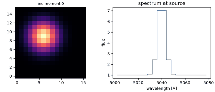
The IFU example scans a synthetic galaxy with an emission line at 5040 Å in sixteen exposures of sixteen slices, then drizzles them onto a 16 × 16 × 20 cube. The line peak, the continuum, and the moment-0 centroid are recovered within one bin and 0.01 pixel.

Real Data: A MaNGA Cube¶

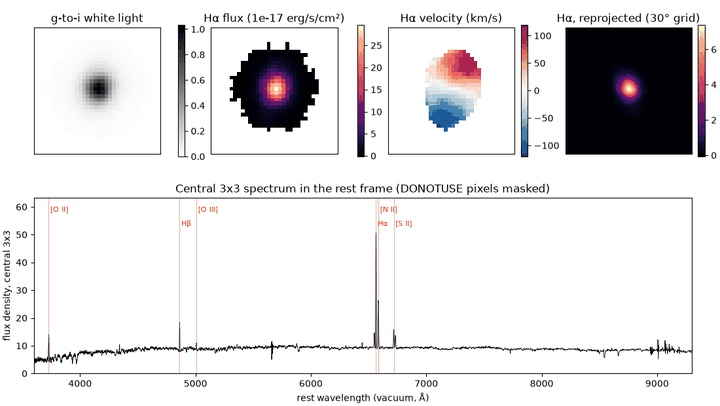
Pipeline cubes do not need coadd_cube to exist, only to be reprojected. The MaNGA example reads the SDSS DR17 cube of the star-forming disc galaxy 8485-1901 (34 × 34 spaxels of 0.5 arcsec, 4563 channels from 3622 to 10354 Å) with torchfits. The steps:

• Spectral axis. The cube's WAVE-LOG axis is evaluated through the 3D WCS and agrees with the file's own WAVE table to 2e-4 Å. Channel edges come from the same WCS at half-pixel positions.
• Rest frame. The redshift is measured on the central Hα line (z = 0.0408). Every spaxel is rebinned onto a 1 Å rest-frame grid with flux_conserving_rebin, which propagates the inverse variance and the DONOTUSE mask.
• Line maps. A continuum from two sidebands is subtracted, which gives the Hα flux map, its 5σ detections (254 spaxels), the Hα centroid velocity field (±100 km/s of ordered rotation) and an integrated [N II]/Hα of 0.41, typical of star formation.
• Reprojection. The continuum-subtracted Hα planes are reprojected with coadd_cube onto a 0.25 arcsec grid rotated by 30°, with Lanczos3 and semantics="flux". The integrated Hα flux is unchanged to 1e-4.

# fragment: path points at the cached manga-8485-1901-LOGCUBE.fits.gz
import torch
import torchfits

from torchsky.spectral import DataCube, SpectralAxis, flux_conserving_rebin
from torchsky.wcs import WCS

header = dict(torchfits.read_header(path, "FLUX"))
flux = torchfits.read(path, hdu="FLUX").double()                  # (4563, 34, 34)
nz = flux.shape[0]
wcs = WCS(header)                                                 # RA---TAN, DEC--TAN, WAVE-LOG
def wavelength(channel):                                          # spectral world coordinate
    return wcs.pixel_to_world(torch.stack([channel * 0 + 16.5, channel * 0 + 16.5, channel], -1))[:, 2]

centres = wavelength(torch.arange(nz, dtype=torch.float64))
edges = wavelength(torch.arange(nz + 1, dtype=torch.float64) - 0.5)
cube = DataCube(data=flux, spectral_axis=SpectralAxis(centres, "Angstrom", "WAVE"))

z = 0.0408
rest = flux_conserving_rebin(flux.permute(1, 2, 0) * (1 + z), edges / (1 + z),
                             torch.arange(6500.0, 6631.0, 1.0, dtype=torch.float64))

Real Data: A MaNGA Cube From Its Fibres¶

The fibre-to-cube example builds the same galaxy's cube from scratch, from its row-stacked spectra (the DR17 LOGRSS file): 19 fibres × 9 dithered exposures. These become one IFU frame (wavelength × fibre):

• Geometry. An IFUSliceWCS holds each fibre's RA and Dec at every wavelength, including differential refraction, and each fibre is its own slice.
• Units. Fibre fluxes are divided by the fibre area to give surface brightness.
• Resampling. The 6400–7000 Å window goes onto 1 arcsec spaxels with the emsm (exponential modified Shepard) kernel.

# fragment: ra, dec, wave are (n_wave, n_fibre) maps from IFURA/IFUDEC, XPOS/YPOS and WAVE
from torchsky.map import CubeTarget, Observation, coadd_cube
from torchsky.wcs import IFUSliceWCS

ifu = IFUSliceWCS(ra_map=ra, dec_map=dec, wavelength_map=wave, slice_id_map=fibre_id)
frame = Observation(data=flux / fibre_area, ifu_wcs=ifu, mask=good, weight=good.float())
cube = coadd_cube([frame], CubeTarget(spatial_wcs=wcs_1arcsec, spectral_bin_edges=edges),
                  spectral_kernel="emsm", emsm_scale=1.0)

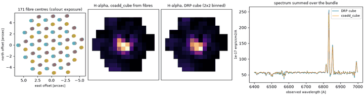
Against the released cube, summed 2 × 2 onto the same grid:

• Flux. The total flux in the window agrees to 1.2 %.
• Position. The image centroids agree to 0.01 spaxel.
• Images. The continuum and Hα images correlate at 0.998 and 0.997.

The weights must be equal per sample, as in the pipeline. Inverse-variance weights favour the fainter fibre of each overlapping pair, because its Poisson noise is lower, and bias this cube 17 % low.

Exact Fibre Footprints¶

emsm reproduces the pipeline because the pipeline uses a similar Shepard kernel. To drizzle each fibre as what it is, a 2 arcsec disk, give the footprint explicitly. Each spaxel then receives the fibre's flux in proportion to the exact overlap area of the disk with it:

# fragment: same sb (surface brightness), ifu, good and target as above
from torchsky.map import IFUObservation, coadd_cube

frame = IFUObservation(sci=sb, detector_to_world=ifu, weight=good.float(),
                       aperture_diameter_arcsec=2.0)
cube = coadd_cube([frame], target, spectral_kernel="drizzle")

On the same MaNGA data the total flux agrees with the DRP cube to 1.1 % and the integrated spectrum to 0.74 % rms, against 2.5 % with emsm. The Hα image is less smooth than the pipeline's Shepard-kernel image, so it correlates with it at 0.981 instead of 0.997. aperture_diameter_arcsec takes one value or one per sample. Without a footprint, drizzle takes each sample's extent from its neighbours in the same slice, and raises when a sample has none, as a fibre does.

Which Path Am I On?¶

Mixing Observation and IFUObservation in one call raises: a cube has one detector model.

Recipes¶

Build a cube from filter images¶

import torch

from torchsky.map import Observation, ResampleConfig, coadd_cube, plan_cube

header = {
    "NAXIS": 2, "NAXIS1": 16, "NAXIS2": 16,
    "CTYPE1": "RA---TAN", "CTYPE2": "DEC--TAN",
    "CRPIX1": 8.5, "CRPIX2": 8.5, "CRVAL1": 150.0, "CRVAL2": 2.0,
    "CDELT1": -0.001, "CDELT2": 0.001,
}
bands = [5000.0, 6000.0, 7000.0]                 # Angstrom
observations = [
    Observation(
        data=torch.full((16, 16), 1.0 + 0.5 * i), wcs=header, wavelength=wavelength,
        weight=1.0, weight_is_inverse_variance=True,
    )
    for i, wavelength in enumerate(bands)
]

target = plan_cube(observations, spectral_axis=bands)
cube = coadd_cube(observations, target, resample=ResampleConfig(semantics="surface_brightness"))

assert tuple(cube.data.shape) == (3, 16, 16)
assert [round(float(v), 2) for v in cube.data[:, 8, 8]] == [1.0, 1.5, 2.0]

plan_cube derives a spatial grid that covers the observations and records the spectral axis and bin edges.

Build a cube from IFU frames¶

An IFUSliceWCS gives the RA, Dec, wavelength, and slice number of every detector pixel. With an explicit CubeTarget (spatial WCS plus spectral bin edges) the output grid is fixed in advance:

import torch

from torchsky.map import CubeTarget, Observation, ResampleConfig, coadd_cube
from torchsky.wcs import WCS, IFUSliceWCS

header = {
    "NAXIS": 2, "NAXIS1": 16, "NAXIS2": 16,
    "CTYPE1": "RA---TAN", "CTYPE2": "DEC--TAN",
    "CRPIX1": 8.5, "CRPIX2": 8.5, "CRVAL1": 150.0, "CRVAL2": 2.0,
    "CDELT1": -0.001, "CDELT2": 0.001,
}
n_wave, n_slice = 12, 16
rows = torch.arange(n_wave, dtype=torch.float64)
cols = torch.arange(n_slice, dtype=torch.float64)

def per_pixel(values_along_axis, axis):
    return values_along_axis.unsqueeze(axis).expand(n_wave, n_slice).clone()

ifu_wcs = IFUSliceWCS(
    ra_map=per_pixel(150.0 + (cols - 7.5) * 0.001, 0),
    dec_map=torch.full((n_wave, n_slice), 2.0, dtype=torch.float64),
    wavelength_map=per_pixel(5000.0 + 2.0 * rows, 1),
    slice_id_map=per_pixel(cols.to(torch.int64), 0),
)
frame = Observation(
    data=torch.ones(n_wave, n_slice), ifu_wcs=ifu_wcs,
    weight=torch.ones(n_wave, n_slice), weight_is_inverse_variance=True,
)

target = CubeTarget(spatial_wcs=WCS(header), spectral_bin_edges=[4980.0, 5000.0, 5020.0, 5040.0])
cube = coadd_cube([frame], target, resample=ResampleConfig(spectral_kernel="drizzle", spectral_pixfrac=0.8))
assert cube.data.shape == (3, 16, 16)

cube.data is (n_wave, y, x), cube.weight the matching weights, cube.spectral_axis the target axis, and cube.header the spatial header. cube.to_data_cube() returns a DataCube for spectral analysis.

Use a physical IFU product¶

For instrument products, construct IFUObservation with the science image, a detector_to_world transform, a DQ plane, slice ids, optional detector pixel footprints, and named variance_components (for example Poisson and read noise). build_ifu_cube returns the science cube, a DQ cube, a usability mask, the explicit voxel covariance, and the response plan that produced them.

Choose a spectral kernel¶

Kernel, spectral_pixfrac, and value semantics (surface_brightness or flux) are recorded in cube.provenance.

Irregular spectral axes¶

Target axes are used as given, including non-uniform ones; non-increasing axes are rejected. The spectral kernels work in bin-index space, so on a strongly irregular axis they bias values near bin edges by about \((\Delta\lambda_{\rm right} - \Delta\lambda_{\rm left})\,\partial F/\partial\lambda\). The bias is small for regular or logarithmic axes; use nearest when exact bin assignment matters more than smoothness.

Uncertainty and covariance¶

cube.inverse_variance is the diagonal voxel inverse variance, present only when every input weight is declared inverse variance. One detector pixel spread over several voxels makes neighbouring voxels correlated, and that covariance is not stored. cube.correlation_factor reports the local ratio to correct aperture errors; build_ifu_cube returns the explicit covariance when you need exact voxel correlations.

Bound memory¶

Observations are processed one at a time, so peak memory is the cube plus one resampled frame. response_chunk_size, max_response_entries, and footprint_max_depth in ResampleConfig bound the IFU response tables; lower them on small devices, raise them when many slices overlap one voxel.

Pitfalls¶

• Wavelength units. Bin edges and wavelength maps must share a unit (Ångström by default); edges in another unit place every pixel in the wrong bin or outside the cube.
• Voxel size against sampling. A spectral bin narrower than the detector sampling leaves empty planes; a spatial pixel smaller than the slice width needs several dithers, as in 2D drizzle.
• MPS. The 3D drizzle and spectral resamplers need float64; use CPU or CUDA.

See Also¶

• Resampling and Coadds for the 2D methods.
• Spectral axes for SpectralAxis, rebinning, and writing cubes with torchfits.
• HEALPix mapmaking for spherical products.
• Reference: coadd_cube, CubeResult.
• Examples: MaNGA cube: Hα map, rotation and reprojection, MaNGA cube rebuilt from its fibre spectra, IFU frames to a spectral cube.