Multi-order coverage (MOC)
A MOC (Multi-Order Coverage map, IVOA standard 2.0) records which parts of
the sky a survey, an image, or a localization covers, with no values attached.
It is a set of HEALPix NESTED cells of mixed orders: large cells
fill the interior of a footprint and small cells trace its edge, so the memory
cost follows the length of the boundary, not the area.
MOC builds coverage from
shapes, images, and catalogs; tests points and pixels against it; combines
footprints with set algebra; and reads and writes the IVOA formats.
How It Works
A cell at order \(k\) (nside \(= 2^k\)) with NESTED index \(p\) is stored as
one integer, its UNIQ number:
The leading term encodes the order, so cells of all orders share one sorted integer space. Internally a MOC is also a list of half-open ranges of NESTED indices at its maximum order: a coarse cell at order \(k\) is the range of its \(4^{(k_\mathrm{max} - k)}\) descendants. Union, intersection, and difference are merges of sorted range lists, and point containment is a binary search.
flowchart LR
    S["shape, WCS image,<br/>or catalog points"] -->|"from_circle, from_polygon,<br/>from_wcs, from_lonlat"| M["MOC<br/>(sorted UNIQ cells)"]
    M -->|"| & −"| M2["combined footprint"]
    M2 -->|"contains, contains_pixels,<br/>overlap_fraction"| Q["boolean masks"]
    M2 -->|"to_sparse_map, flatten"| D["fixed-order pixels"]
    M2 -->|"to_ascii, to_json, write_fits"| F["IVOA interchange"]
max_order fixes the resolution of the boundary. At order 10 (3.4 arcmin
cells) a footprint edge is uncertain by up to one cell; at order 16 it is
3.2 arcsec. Constructors cover a cell when any part of it overlaps the shape,
so a MOC is a superset of the exact region, larger by roughly half a cell
along the boundary.
When to Use It
| You have | Use |
|---|---|
| Coverage only: survey footprints, exposure unions, cross-match pruning | MOC |
| Values at one resolution where data exist (depth, weight, counts) | SparseHealpixMap |
| Values whose resolution follows the signal (GW or neutrino localizations) | MultiOrderHealpixMap |
| An exact polygon or cap for geometry, not pixels | SphericalPolygon |
| A genuinely full-sky field that fits in memory | A dense tensor |
Minimal Example: The Footprint of a MegaPipe Cutout
The header below is the real WCS of a 512 × 512 CFHT MegaPipe cutout (sample
cadc_megapipe_cutout, see Projections).
MOC.from_wcs turns the pixel grid into coverage; the exact area of the
footprint polygon shows how much the boundary cells add.
import math

import torch

from torchsky.sphere import MOC, spherical_polygon_area
from torchsky.wcs import WCS

wcs = WCS({  # CFHT MegaPipe 712.165, g band, CADC cutout
    "NAXIS": 2, "NAXIS1": 512, "NAXIS2": 512,
    "CTYPE1": "RA---TAN", "CTYPE2": "DEC--TAN",
    "CRVAL1": 359.07190997, "CRVAL2": -7.5, "CRPIX1": -2999.0, "CRPIX2": 1001.0,
    "CD1_1": -5.160234650248e-05, "CD1_2": 0.0, "CD2_1": 0.0, "CD2_2": 5.160234650248e-05,
})
moc = MOC.from_wcs(wcs, shape=(512, 512), max_order=16)        # 3.2 arcsec cells

corners = wcs.footprint(shape=(512, 512))
exact_arcmin2 = float(spherical_polygon_area(corners[:, 0], corners[:, 1])) * (180 / math.pi) ** 2 * 3600
moc_arcmin2 = moc.area_sq_deg * 3600
assert 1.0 < moc_arcmin2 / exact_arcmin2 < 1.15                # boundary cells add ~8%

centre = wcs.pixel_to_world(torch.tensor([255.5], dtype=torch.float64),
                            torch.tensor([255.5], dtype=torch.float64))
assert bool(moc.contains(*centre).all())
assert moc.to_ascii(compact=True).startswith("13/")           # coarsest cells are order 13
Real footprints are larger and the overhead smaller: the Horsehead WCS tour builds the order-15 MOC of a 15 × 15 arcmin DSS plate in 674 cells, 2% above the exact area. The Chandra example builds coverage from the events themselves:
# fragment: ra, dec are the event positions from the Chandra example
from torchsky.sphere import MOC

moc = MOC.from_lonlat(ra, dec, max_order=12)   # 132 cells, 420 arcmin^2, five ACIS chips
assert bool(moc.contains(ra, dec).all())
Real Data: Survey Footprints
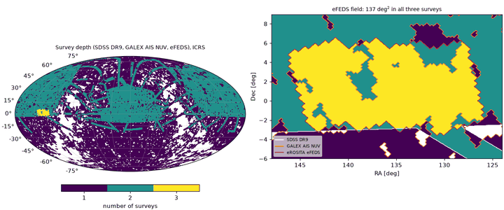
Surveys publish their coverage as MOC files. The footprint example combines the SDSS DR9, GALEX AIS NUV, and eROSITA eFEDS coverage MOCs:
# fragment: sdss, galex, efeds = MOC.read_fits(...) on the published MOC files
both = sdss & galex                      # 12994.4 deg^2
either = sdss | galex                    # 34538.5 deg^2 = 14693.1 + 32839.7 - 12994.4
triple = both & efeds                    # 137.0 deg^2 of the 159.7 deg^2 eFEDS field
Areas count cells at the deepest order, so inclusion–exclusion holds exactly.
MOC.read_fits reads IVOA MOC files as published by CDS: the UNIQ table in
the extension named MOC, or else in the first extension with
ORDERING = 'NUNIQ'. Time MOCs and non-ICRS coverage raise.
Recipes
Build Coverage from Shapes
import torch

from torchsky.sphere import MOC

circle = MOC.from_circle(10.0, 20.0, 1.0, max_order=8)      # lon, lat, radius in degrees
square = MOC.from_polygon(torch.tensor([0.0, 2.0, 2.0, 0.0]),
                          torch.tensor([0.0, 0.0, 2.0, 2.0]), max_order=6)
points = MOC.from_lonlat(torch.tensor([15.0, 16.0]), torch.tensor([-3.0, 4.0]), max_order=6)

assert circle.contains(torch.tensor([10.0, 200.0]), torch.tensor([20.0, -40.0])).tolist() == [True, False]
assert bool(square.contains(torch.tensor(1.0), torch.tensor(1.0)))
assert circle.area_sq_deg > 4.5                             # 13.7' cells inflate a 1-degree disc
fine = MOC.from_circle(10.0, 20.0, 1.0, max_order=12)        # 0.86' cells
assert 3.14 < fine.area_sq_deg < 3.3                          # close to pi square degrees
Coverage constructors are hierarchical: interior cells stay coarse and only
the boundary is subdivided to max_order. Other entry points:
from_region (any
torchsky region or a PixelizedRegion, kept at its resolution),
from_sparse_map,
from_threshold
(pixels of a sparse map above or below a value), MOC.empty(), and MOC.full().
Combine Footprints
MOCs are closed under union (|), intersection (&), and difference (-),
across cells of different orders. overlaps answers "do these intersect?"
without building the intersection; contains_moc is the subset test.
import torch

from torchsky.sphere import MOC

a = MOC.from_circle(0.0, 0.0, 2.0, max_order=6)
b = MOC.from_circle(3.0, 0.0, 2.0, max_order=6)

assert a.overlaps(b)
union, both, only_a = a | b, a & b, a - b
assert both.area <= min(a.area, b.area) <= max(a.area, b.area) <= union.area
assert abs(union.area - (a.area + b.area - both.area)) < 1e-12

assert union.degrade(4).max_order <= 4         # coarser, still a superset
mask = a.flatten(64)                           # dense boolean NESTED mask, 12 * 64**2
assert mask.dtype == torch.bool and mask.numel() == 12 * 64**2
On CPU the set operations, UNIQ-to-range conversion, and degrade run in
small native kernels over the range lists; CUDA and MPS use the torch
implementation, which is also the parity oracle in the tests.
Filter a Catalog or an Indexed Table
contains(lon, lat) returns a boolean mask that broadcasts over tensors and
allocates no dense map; index the catalog with it. For rows that already carry
HEALPix indices, contains_pixels(nside, pixels, nest=True) skips the
trigonometry, and overlap_fraction(uniq) reports how much of a cell is
covered. Catalog.inside(moc) does the same for a
catalog object, and sample_randoms draws points uniformly inside the
coverage for random catalogs.
Save and Exchange
MOC serialization follows the IVOA standard: ASCII (order/pixel ranges),
JSON, and FITS. FITS goes through torchfits (write_fits, read_fits).
import torch

from torchsky.sphere import MOC

moc = MOC.from_circle(120.0, -30.0, 0.5, max_order=7)
text = moc.to_ascii(compact=True)
restored = MOC.from_ascii(text)
assert abs(restored.area - moc.area) < 1e-12
assert abs(MOC.from_json(moc.to_json()).area - moc.area) < 1e-12
assert bool(restored.contains(torch.tensor(120.0), torch.tensor(-30.0)))
from_mocpy/to_mocpy convert at a boundary when mocpy is installed; mocpy is
never a runtime backend.
Add Time: STMOC
STMOC (MOC 2.0 space-time
coverage) pairs spatial cells with time cells of 1 µs resolution since
JD = 0. Use it for exposure windows, transient searches, and time-filtered sky
queries.
from torchsky.sphere import MOC, STMOC

field = MOC.from_circle(10.0, 0.0, 1.0, max_order=6)
night = STMOC.from_spatial_coverages(59000.0, 59001.0, field, time_depth=16)   # MJD window

assert bool(night.contains(59000.5, 10.0, 0.0))
assert not bool(night.contains(60000.0, 10.0, 0.0))
assert night.query_by_time(59000.0, 59000.5).area > 0.0
from_times_positions quantizes catalog samples onto time × HEALPix cells;
mjd_to_time_us and time_us_to_mjd convert to the STMOC time axis. BMOC
is the boundary-flagged variant for footprints that need their edge cells
marked.
Accuracy and Validation
Constructors, set algebra, and serialization agree with mocpy in torchsky-harness; see the parity page. In the test suite the native range kernels are compared with the torch path.
Pitfalls
- A MOC is a superset. Its area exceeds the exact region by about half a
boundary cell per unit length of edge. Use
spherical_polygon_areawhen you need the exact area. max_orderis a resolution, not a precision knob for free. Each extra order roughly doubles the number of boundary cells.flattenandto_denseallocate full-sky arrays. Call them once, at the boundary, not inside a loop.nest2uniqtakesnside, not order:nest2uniq(nside, pixels).
See Also
- HEALPix, Sparse maps, Celestial sphere overview.
- Catalogs: footprint selection and crossmatch pruning.
- Reference:
MOC,STMOC,nest2uniq. - Examples: HEALPix and MOC, Chandra events, Planck power spectrum (a Galactic-cut MOC gives \(f_\mathrm{sky}\) exactly), survey footprints.