Scenes¶

A scene is a description of the sky on a chosen target: a pixel grid with a WCS and a declared value semantics (surface brightness or flux per pixel). Each recorded exposure is linked to the scene by an observation operator \(A\), a linear map that predicts the exposure's pixels from the scene: resampling from the target grid to the detector, and optionally PSF, bandpass, and background. With several exposures \(A_1, \dots, A_N\), the scene that best explains all of them under Gaussian noise solves the normal equations

where \(y_n\) are the data, \(N_n\) the noise covariance, and \(A_n^\mathsf{T}\) the adjoint (transpose) of each operator, which spreads pixel residuals back onto the scene.

torchsky.scene builds targets from headers, wraps exposures in operators whose adjoints are exact, and solves the normal equations matrix-free with conjugate gradients (CG): \(A\) and \(A^\mathsf{T}\) are applied as functions, and no matrix is ever formed. Use it for image-plane inversion of dithered exposures (a statistically optimal alternative to a coadd), for forward modelling with your own scene representation, and as the operator layer under fields and likelihoods.

How It Works¶

flowchart LR
    T["target<br/>(header, value semantics)"] --> B["bind"]
    O["ImageObservation<br/>(pixels, WCS, weight)"] --> AD["operator adapter"]
    AD --> B
    B --> A["bound operator A<br/>apply · apply_adjoint · noise"]
    A --> S["solve AᵀN⁻¹A x = AᵀN⁻¹y<br/>(CG, matrix-free)"]
    A --> G["or autograd through A"]

operator_adapter_for_observation wraps one exposure with the same resampling kernels used by coadds; bind_image_plane_target fixes the target and returns a bound operator with apply, apply_adjoint, and the inverse-noise weighting from the exposure's weight and mask. To start from a FITS file, scene.image_observation reads the image and header with torchfits. The adjoint is the exact vector–Jacobian product of the forward projection, so \(\langle A u, v\rangle = \langle u, A^\mathsf{T} v\rangle\) holds to floating-point rounding, and CG converges to the true least-squares solution rather than to that of a nearby, inconsistent operator.

Assumptions and Accuracy¶

• Operators are linear in the scene with their parameters fixed. Nonlinear instrument effects need autograd instead of the normal equations.
• The weight maps are inverse variances. Rescaled or clipped weights still give a weighted least-squares solution but not a calibrated likelihood.
• Pixels on the target that no exposure constrains make the normal operator singular. Add damping, a prior, or restrict the target.
• Adjoint identities are checked by dot-product tests, and CG against dense solves, in the test suite.

A Dot-Product Test and a Solve¶

import torch

from torchsky import scene
from torchsky.map import ImageObservation

header = {
    "NAXIS": 2, "NAXIS1": 32, "NAXIS2": 32,
    "CTYPE1": "RA---TAN", "CTYPE2": "DEC--TAN",
    "CRPIX1": 16.5, "CRPIX2": 16.5, "CRVAL1": 150.0, "CRVAL2": 2.0,
    "CDELT1": -0.05 / 3600.0, "CDELT2": 0.05 / 3600.0,
}
target = scene.target_from_header(header, value_semantics="surface_brightness")
yy, xx = torch.meshgrid(torch.arange(32.0), torch.arange(32.0), indexing="ij")
sky = torch.exp(-((xx - 16) ** 2 + (yy - 16) ** 2) / 18.0)

shifted = {**header, "CRVAL1": 150.0 + 0.4 * 0.05 / 3600.0}      # 0.4 pixel offset
operator = scene.operator_adapter_for_observation(
    ImageObservation(data=sky, wcs=shifted), resampling_kernel="bilinear"
).bind_image_plane_target(target)

u, v = torch.randn(32, 32), torch.randn(32, 32)
torch.testing.assert_close((operator.apply(u) * v).sum(), (u * operator.apply_adjoint(v)).sum(), rtol=1e-4, atol=1e-4)

solved = operator.solve_normal_equation_cg(operator.apply(sky), iterations=8)
assert solved.solution.shape == sky.shape

The MegaPipe mosaic example uses the same resampling kernels in forward (coadd) form.

Real Data: Forced Photometry of Gaia Stars¶

A scene does not have to be a pixel grid. A SourceCatalogScene is a list of sources at fixed sky positions with one flux per band, rendered through each observation's WCS and PSF. Its parameters enter the prediction linearly, so fitting them is an exact linear least-squares problem. fit_forced_photometry groups stars whose footprints overlap and solves each group for its fluxes and a local background on the native pixels.

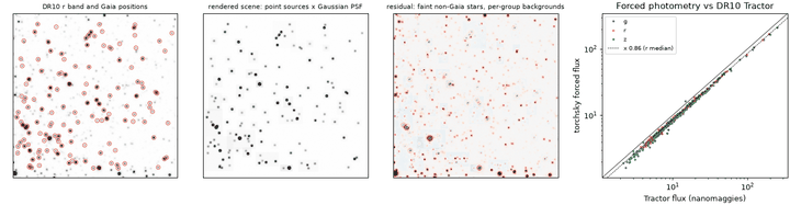
The forced photometry example does this on a 100 arcsec Legacy Surveys DR10 g/r/z cutout 4 arcmin from the globular cluster NGC 288. It uses the 143 Gaia stars in the DR10 Tractor catalogue of the field. The PSF is a Gaussian whose width is fitted per band by minimising chi-square over a grid of widths, giving FWHM 1.29, 0.98 and 0.86 arcsec in g, r and z.

# fragment: images, invvar, header, ra, dec and sigma come from the cached cutout and catalogue
import torch

from torchsky.catalogs import fit_forced_photometry
from torchsky.field import FieldObservation, PSFSpec
from torchsky.scene import SourceCatalogScene

observations = [
    FieldObservation(image=images[k], header=header, weight=invvar[k],
                     band_name=band, psf_spec=PSFSpec.gaussian(sigma[k]))
    for k, band in enumerate("grz")
]
scene = SourceCatalogScene(ra, dec, coefficients=torch.zeros((ra.numel(), 3), dtype=torch.float64),
                           band_labels=("g", "r", "z"))
result = fit_forced_photometry(observations, scene, background="constant")
# result.flux: (143, 3) nanomaggies; result.predictions: the rendered scene per band

The forced fluxes follow the Tractor fluxes star by star with a robust scatter of 3 % in every band. Their median ratio, 0.82–0.86, is an aperture correction, not an error: Tractor fits pixelized PSF models with extended wings to the individual exposures, and a Gaussian core misses that light. Use a measured PSF (a kernel PSFSpec or a template morphology) when absolute fluxes matter. The residual image also shows what a forced fit cannot do: stars missing from the input catalogue stay in the data, and each blend group absorbs them into its local background. A full fit of all 143 stars and three bands takes about a second on a CPU.

Recipes¶

Invert Several Dithered Exposures¶

bind_image_plane_observations_to_target binds a list of exposures to one target. The normal operator sums over them in exposure order; exposure_chunk_size caps how many predictions are held in memory at once. Four half-pixel dithers recover the scene to rounding error:

import torch

from torchsky import scene
from torchsky.map import ImageObservation

header = {
    "NAXIS": 2, "NAXIS1": 24, "NAXIS2": 24,
    "CTYPE1": "RA---TAN", "CTYPE2": "DEC--TAN",
    "CRPIX1": 12.5, "CRPIX2": 12.5, "CRVAL1": 150.0, "CRVAL2": 2.0,
    "CDELT1": -0.1 / 3600.0, "CDELT2": 0.1 / 3600.0,
}
target = scene.target_from_header(header, value_semantics="surface_brightness")
yy, xx = torch.meshgrid(torch.arange(24.0), torch.arange(24.0), indexing="ij")
sky = torch.exp(-((xx - 12) ** 2 + (yy - 12) ** 2) / 8.0)

dithers = [(0.0, 0.0), (0.5, 0.0), (0.0, 0.5), (0.5, 0.5)]
exposures = [
    ImageObservation(data=torch.zeros(24, 24), wcs={**header, "CRPIX1": 12.5 + dx, "CRPIX2": 12.5 + dy})
    for dx, dy in dithers
]
operators = scene.bind_image_plane_observations_to_target(exposures, target, resampling_kernel="bilinear")
data = operators.apply(sky)                     # one predicted image per exposure
result = operators.solve_normal_equation_cg(data, iterations=50, damping=1e-6)
assert (result.solution - sky)[4:-4, 4:-4].abs().max() < 1e-4

result.residual_norm_history and result.diagnostics report convergence; solve_least_squares_lsqr is available when the normal operator is singular.

Fit by Gradient Descent Instead¶

The same bound operator is differentiable, so a nonlinear loss or a prior that the normal equations cannot express is an ordinary PyTorch loop. The models overview fits a sky through one operator with Adam.

Bring Your Own Forward Model¶

adapter.bind_target(target, apply_operator=..., apply_adjoint=..., apply_noise=...) binds any linear forward model you supply. The adjoint is then your responsibility: check it with the dot-product test above before solving. A BoundObservationOperator built this way also feeds a GaussianLikelihoodFactor.

Other Scene Representations¶

SceneRepresentation adapters let the same observation path render a tensor grid (DiscreteTargetImage), a HEALPix map (HealpixMapScene), spherical-harmonic coefficients (HarmonicAlmScene), a fitted field (ContinuousFieldModel), or a list of point, Gaussian, or Sérsic sources (SourceCatalogScene). scene.render and scene.predict dispatch on the representation.

Approximate Pixel Uncertainties¶

An operator set estimates the diagonal of \((H + \epsilon I)^{-1}\), with \(H = \sum_n A_n^\mathsf{T} N_n^{-1} A_n\), by random probing (Hutchinson's estimator), each probe solved by CG:

# fragment: operators from bind_image_plane_observations_to_target, reference_map a target-shaped tensor
inverse_curvature = operators.estimate_posterior_variance_diagonal(
    reference_map, num_probes=64, seed=7, iterations=32, damping=1.0e-6,
)

Despite the method name, this is the diagonal of the inverse curvature, which equals a posterior variance only for a well-posed, unregularized Gaussian problem. Finite-probe estimates are noisy and can be negative; they are returned signed because clipping would bias them. Every probe solve is checked, and a failed solve raises instead of returning a number.

Pitfalls¶

• Declare value semantics. Surface brightness is independent of pixel size; flux per pixel scales with pixel area. A mismatch between target and data changes the solution by the pixel-area ratio.
• Unconstrained pixels. Target pixels outside every exposure, or under masks in all of them, have no data; damp them or crop the target.
• CG iterations are not convergence. Read the residual history, and check that a tighter tolerance leaves the result unchanged.
• Noise correlations. Resampled inputs have correlated noise. Invert the native exposures, not coadds of them.

See Also¶

• Likelihoods: Gaussian and Poisson–Gaussian factors on bound operators.
• Fields: continuous scene models through the same operators.
• Resampling: the kernels inside the operators.
• Reference: torchsky.scene, torchsky.map.solvers.
• Example: forced photometry of Gaia stars on Legacy Surveys images.