Synthetic photometry¶

Synthetic photometry predicts what an imaging camera would measure for a source with a known spectrum: the spectrum is weighted by the filter's passband (its throughput \(R(\lambda)\), the fraction of photons transmitted at each wavelength) and averaged into a single flux or magnitude. torchsky.spectrophotometry does this on tensors: a Passband is two tensors, a spectrum is a tensor with any number of leading batch dimensions, and the result carries its value, unit, coverage, and valid flag. The integral is differentiable with respect to the spectrum, so magnitudes can sit inside a fitting loss.

Use it to compare spectra with catalogue photometry, to compute colours of model spectral energy distributions (SEDs) across redshift, and to calibrate spectra against imaging.

How It Works¶

A CCD counts photons, so each wavelength is weighted by its photon rate, \(F_\lambda \lambda / hc\). The photon-weighted mean flux density in a band is

\[ \langle F_\lambda \rangle = \frac{\int F_\lambda(\lambda)\, R(\lambda)\, \lambda\, \mathrm d\lambda} {\int R(\lambda)\, \lambda\, \mathrm d\lambda}, \qquad \langle F_\nu \rangle = \frac{\int F_\lambda\, R\, \lambda\, \mathrm d\lambda} {c \int R / \lambda\, \mathrm d\lambda}, \]

and the AB magnitude is \(m_\mathrm{AB} = -2.5 \log_{10}(\langle F_\nu\rangle / 3631\,\mathrm{Jy})\): a source with constant \(F_\nu = 3631\) Jy has magnitude zero in every band.

The integrals are evaluated on the union of the spectrum and passband samples over their common range. Both curves are interpolated linearly onto that grid and integrated with the trapezoid rule, so no sample of either curve is skipped. Coverage is the fraction of the passband's photon weight \(\int R\lambda\,\mathrm d\lambda\) that falls on valid spectrum samples. Below min_coverage (default 0.99) the result is NaN with valid=False; nothing is extrapolated or renormalized.

flowchart LR
    S["spectrum F_λ<br/>+ mask"] --> U["union grid,<br/>linear interpolation"]
    B["passband R(λ)"] --> U
    U --> I["trapezoid integrals<br/>photon weight R·λ"]
    I --> C{"coverage ≥<br/>min_coverage?"}
    C -->|yes| V["mean F_λ, μJy, or AB mag"]
    C -->|no| N["NaN, valid=False"]

Assumptions and Accuracy¶

Wavelengths are vacuum Angstrom inside the module; wavelength_unit="nm" converts once at construction.
output="mean_f_lambda" works in any flux unit per Angstrom. "f_nu_microjy" and "ab_mag" require cgs \(F_\lambda\) (erg s⁻¹ cm⁻² Å⁻¹).
Throughput is a dimensionless photon response. Detector quantum efficiency and atmosphere belong in the curve if they are part of the system response; collecting area and exposure time belong in the flux calibration.
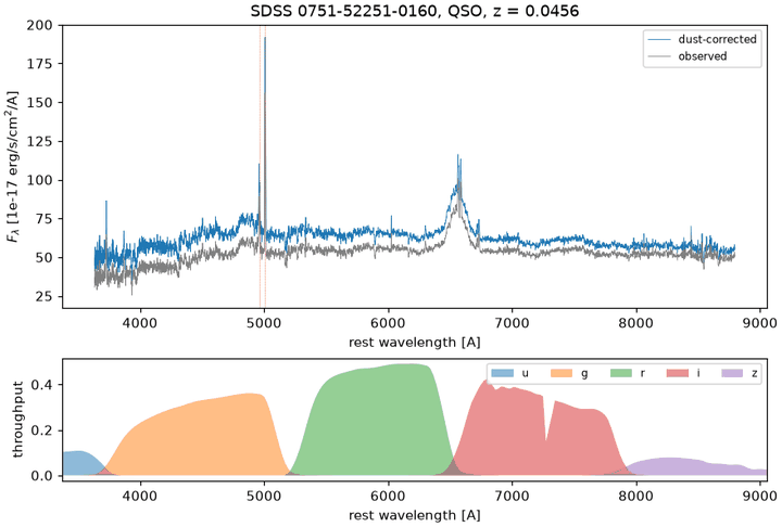
A constant \(F_\lambda\) or \(F_\nu\) is recovered exactly by construction. On the real SDSS spectrum below, the g, r, and i magnitudes agree with the synthetic magnitudes of the SDSS pipeline to 0.03 mag (0.017 mag rms).

A Real Spectrum Through SDSS Filters¶

Integrate the calibrated SDSS spectrum of plate 0751, fibre 160 through the SDSS r passband from the SVO Filter Profile Service:

# fragment: needs spec-0751-52251-0160.fits and SDSS.r.dat (SVO "SLOAN/SDSS.r", ASCII)
import torch
import torchfits

from torchsky.filter_profiles import bandpass_from_transmission_file
from torchsky.spectrophotometry import Passband, synthetic_photometry

coadd = torchfits.read("spec-0751-52251-0160.fits", hdu=1)
wave = 10.0 ** coadd["loglam"].to(torch.float64)
flux = coadd["flux"].to(torch.float64) * 1e-17          # cgs F_lambda
good = coadd["ivar"] > 0

curve = bandpass_from_transmission_file("SDSS.r.dat", band_name="r")
r = Passband.from_samples(
    curve["transmission_wavelength"].to(torch.float64),
    curve["transmission_throughput"].to(torch.float64),
    name="r",
)
mag = synthetic_photometry(wave, flux, r, output="ab_mag", mask=good, min_coverage=0.9)
print(mag.value, mag.coverage, mag.valid)    # 16.776, 1.00, True (SDSS pipeline: 16.764)

The spectrum covers 3800–9200 Å, so u (12 per cent of its photon weight) and z (69 per cent) are reported invalid. The figure shows the spectrum and the five passbands; the full script is examples/sdss_spectrum_photometry.py.

SDSS quasar spectrum with ugriz passbands

Recipes¶

Get a Passband¶

Source	Function
Two-column text file (SVO ASCII, instrument tables)	`bandpass_from_transmission_file`
SVO Filter Profile Service by facility and instrument	`bandpass_from_svo` (needs `astroquery` unless cached)
Gaussian or linear-variable filter	`evaluate_throughput`
Tensors you already have	`Passband`, `Passband.from_samples`

Passband requires strictly increasing wavelengths and non-negative throughput; from_samples sorts an unsorted table and averages duplicate wavelengths. torchsky.filter_profiles is experimental.

import torch

from torchsky.spectrophotometry import Passband

band = Passband.from_samples(
    torch.tensor([600.0, 400.0, 500.0], dtype=torch.float64),
    torch.tensor([0.0, 0.0, 1.0], dtype=torch.float64),
    name="toy",
    wavelength_unit="nm",
)
assert band.wavelength.tolist() == [4000.0, 5000.0, 6000.0]
print(band.effective_wavelength.item(), band.pivot_wavelength.item())

effective_wavelength is photon-weighted; pivot_wavelength converts between \(\langle F_\lambda\rangle\) and \(\langle F_\nu\rangle\) via \(F_\nu = F_\lambda \lambda_\mathrm{p}^2 / c\).

AB Magnitudes of a Batch in Several Bands¶

synthetic_photometry_bands puts bands on a trailing axis. A constant \(F_\nu\) gives the same AB magnitude in every band.

import torch

from torchsky.spectrophotometry import Passband, synthetic_photometry_bands

g = Passband(torch.tensor([4000.0, 5000.0, 6000.0], dtype=torch.float64), torch.tensor([0.0, 1.0, 0.0], dtype=torch.float64))
r = Passband(torch.tensor([5500.0, 6500.0, 7500.0], dtype=torch.float64), torch.tensor([0.0, 1.0, 0.0], dtype=torch.float64))
wave = torch.linspace(4000.0, 7500.0, 351, dtype=torch.float64)

f_nu_cgs = torch.tensor([[1e-28], [1e-29]], dtype=torch.float64)       # two sources
flux_lambda = f_nu_cgs * 2.99792458e18 / wave.square()                  # cgs F_lambda
mags = synthetic_photometry_bands(wave, flux_lambda, [g, r], output="ab_mag")
assert mags.value.shape == (2, 2)
torch.testing.assert_close(mags.value[:, 0], mags.value[:, 1], rtol=1e-6, atol=1e-6)
torch.testing.assert_close(mags.value[1] - mags.value[0], torch.full((2,), 2.5, dtype=torch.float64))

Photon or Energy Weighting¶

CCDs count photons, so the default is photon weighting. Bolometers and some published curves give the response per unit energy, \(R_E\); pass weighting="energy" for the mean \(\int F_\lambda R_E\,\mathrm d\lambda / \int R_E\,\mathrm d\lambda\), and \(\langle F_\nu\rangle = \int F_\lambda R_E\, \mathrm d\lambda / (c \int R_E \lambda^{-2}\,\mathrm d\lambda)\) (Bessell & Murphy 2012). Coverage uses the same weight. A constant \(F_\nu\) has the same AB magnitude in both modes.

import torch

from torchsky.spectrophotometry import Passband, synthetic_photometry

wave = torch.linspace(4000.0, 6000.0, 201, dtype=torch.float64)
response_energy = torch.exp(-0.5 * ((wave - 5000.0) / 300.0) ** 2)
flux = (wave / 5000.0) ** -2.0
band = Passband(wave, response_energy)

energy_mean = synthetic_photometry(wave, flux, band, weighting="energy").value
expected = torch.trapezoid(flux * response_energy, wave) / torch.trapezoid(response_energy, wave)
torch.testing.assert_close(energy_mean, expected)
photon_mean = synthetic_photometry(wave, flux, band).value
assert photon_mean < energy_mean                  # photon weighting favours the red side

Vega Magnitudes¶

vega_zero_point integrates Vega through a band, with the same output and weighting as synthetic_photometry; pass it to flux_to_magnitude. Vega is the STScI CALSPEC spectrum alpha_lyr_stis_012 (Bohlin, Hubeny & Rauch 2020: HST/STIS from 1152 to 10200 Å joined to a model, 900 Å to 300 µm, vacuum wavelengths), public-domain data shipped with torchsky (92 kB) and returned by vega_spectrum. It matches synphot given the same spectrum to \(2\times10^{-6}\).

import torch

from torchsky.spectrophotometry import (Passband, flux_to_magnitude, synthetic_photometry,
                                        vega_spectrum, vega_zero_point)

band = Passband(torch.tensor([4800.0, 5500.0, 6200.0], dtype=torch.float64),
                torch.tensor([0.0, 1.0, 0.0], dtype=torch.float64))
zero = vega_zero_point(band)                     # erg/s/cm2/A
assert 3.4e-9 < float(zero) < 3.8e-9

wave = torch.linspace(4500.0, 6500.0, 401, dtype=torch.float64)
f_nu = 3631e-23 * 10 ** (-0.4 * 10.0)            # an AB = 10 source
ab_source = f_nu * 2.99792458e18 / wave**2
m_vega = flux_to_magnitude(synthetic_photometry(wave, ab_source, band).value, zero_point=zero)
assert abs(float(m_vega) - 9.995) < 1e-3          # Vega is AB = 0.005 in this band

vega_wave, vega_flux = vega_spectrum()
assert abs(float(flux_to_magnitude(synthetic_photometry(vega_wave, vega_flux, band).value, zero))) < 1e-12

Some systems assign Vega a small non-zero magnitude (for example 0.03 in V); add that offset yourself. flux_to_magnitude returns NaN, not -inf, for non-positive fluxes.

Gaps and Coverage¶

Mark missing samples with mask (True means the sample exists) rather than putting NaN in the flux. Masked runs are integrated separately, a hole is never bridged by interpolation, and the hole reduces coverage.

import torch

from torchsky.spectrophotometry import Passband, synthetic_photometry

band = Passband(torch.tensor([4000.0, 5000.0, 6000.0], dtype=torch.float64), torch.tensor([0.0, 1.0, 0.0], dtype=torch.float64))
wave = torch.linspace(4000.0, 6000.0, 21, dtype=torch.float64)
flux = torch.ones_like(wave)
mask = torch.ones_like(wave, dtype=torch.bool)
mask[8:13] = False                                  # a detector gap at the band centre

holed = synthetic_photometry(wave, flux, band, mask=mask)
assert not bool(holed.valid) and torch.isnan(holed.value)
relaxed = synthetic_photometry(wave, flux, band, mask=mask, min_coverage=0.0)
assert float(relaxed.coverage) < 0.7 and torch.isfinite(relaxed.value)

Gaussian and Position-Dependent Filters¶

evaluate_throughput evaluates a Gaussian response in the unit you pass. With lambda_center_map the centre varies with detector position, as in a linear-variable filter.

import torch

from torchsky.spectrophotometry import evaluate_throughput

wave_nm = torch.tensor([500.0, 510.0, 520.0], dtype=torch.float64)
centres = torch.tensor([[500.0], [520.0]], dtype=torch.float64)    # two detector rows
lvf = evaluate_throughput(wave_nm.expand(2, -1), sigma=4.0, lambda_center_map=centres, wavelength_unit="nm")
assert lvf.shape == (2, 3) and lvf[0, 0] > lvf[0, 2] and lvf[1, 2] > lvf[1, 0]

Pitfalls¶

Lowering min_coverage is extrapolation. If a band is not covered, extend the spectrum (or model it) rather than accepting a partial integral.
Units. ab_mag from a spectrum in units of \(10^{-17}\) erg s⁻¹ cm⁻² Å⁻¹ is off by 42.5 mag; scale to cgs first.
Air-wavelength filter curves. Some ground-based curves are tabulated in air. Convert them to vacuum before mixing them with vacuum spectra.
MPS precision. Passbands are float64 on CPU and CUDA; MPS has no float64 and keeps the tensor's float32, with correspondingly lower precision.