HEALPix mapmaking¶

An image-plane coadd describes the sky on one flat grid, tied to a projection and a tangent point. A HEALPix map describes it on the whole sphere: the HEALPix pixelization divides the sky into \(12\,N_{\rm side}^2\) equal-area cells, so a map built from any number of pointings has one pixel layout, no projection distortion, and no edges between tiles. coadd_healpix projects calibrated images directly onto such a map, and resample_healpix takes a map back onto any image WCS.

Use it for products that span many fields or the whole sky, for maps that must be combined with other HEALPix data (Planck, WMAP, survey depth and mask maps), and as input to spherical harmonic analysis. For a single field that you will measure with image tools, a coadd on a TAN grid is simpler.

How It Works¶

flowchart LR
    O["exposure<br/>data, WCS, weight"] --> M["MOC of the<br/>footprint at Nside"]
    M --> P["HEALPix cells<br/>inside the footprint"]
    P -->|"cells finer than<br/>kernel support"| S["interpolate data and<br/>weight at cell centre"]
    P -->|"coarser cells"| I["integrate pixels over<br/>their overlap with each cell"]
    S --> A["accumulate Σ w·d, Σ w<br/>dense or sparse"]
    I --> A
    A --> R["HealpixResult<br/>data, weight, overlap_count,<br/>coverage MOC"]

Values are surface brightness. Each exposure enters in one of two regimes, chosen from the cell size \(L\) (nside2resol) and the exposure's pixel size \(p\) (the square root of the solid angle of its central pixel).

Centre sampling, when \(L \le s\,p\) with \(s\) the kernel support (1 pixel for nearest, 2 bilinear, 4 bicubic and lanczos2, 6 lanczos3, 8 lanczos4). torchsky lists the HEALPix cells inside the footprint, maps each cell centre into the exposure's pixel coordinates, and interpolates data and weight there with the kernel:

\[ M_p = \frac{\sum_k w_k(\mathbf x_{kp})\, d_k(\mathbf x_{kp})}{\sum_k w_k(\mathbf x_{kp})}, \]

with \(\mathbf x_{kp}\) the position of the centre of cell \(p\) in exposure \(k\).

Overlap integration, when \(L > s\,p\) (centre samples would leave image pixels unused) or when the footprint contains no cell centre. Each image pixel \(i\) is shared among the cells it overlaps, as drizzle does at pixfrac = 1:

\[ M_p = \frac{\sum_k \sum_i A_{ip}\, w_{ki}\, d_{ki}}{\sum_k \sum_i A_{ip}\, w_{ki}}, \qquad W_p = \sum_k \sum_i A_{ip}\, w_{ki}, \]

with \(A_{ip}\) the area of pixel \(i\) inside cell \(p\) in units of the cell area. A cell only partly covered by an exposure gets that exposure's mean over the covered part, weighted by the covered fraction; a fully covered cell gets weight \(w\), as in centre sampling. The overlap is computed exactly in HEALPix's equal-area lattice coordinates, where every cell is a unit square: each pixel is the quadrilateral of its projected corners, clipped against the cells and the equatorial or polar zone it falls in. The kernel is not used.

Cells are processed in chunks, so memory is the map plus one chunk. Optional sky= and outliers= configurations work as in coadds.

Assumptions. The map is in ICRS: exposures with Galactic, ecliptic, FK4, or FK5 WCS are converted. An FK5 (J2000) header gets the roughly 20 mas FK5 to ICRS frame bias and emits CelestialFrameBiasWarning, as in the image-plane path; set RADESYS = 'ICRS' if the astrometry was solved against Gaia. Validation. HEALPix indexing matches healpy exactly (parity), and the multiband example checks the map against an analytic sky at every cell centre. The package tests check the overlap weights against an independent 24 × 24 sub-pixel integration to \(2\times10^{-3}\) of a cell, and the total covered area to \(10^{-5}\), including cells that straddle the polar zones, the 0° meridian, and a pole.

Four MegaPipe Cutouts on HEALPix¶

The four CFHT MegaPipe cutouts of the mosaic example (0.186 arcsec pixels) go straight onto a sparse map with 0.40 arcsec cells, without an intermediate flat mosaic:

# megapipe_mosaic_[abcd].fits: examples/megapipe_mosaic.py downloads them from CADC.
import torch
import torchfits

from torchsky.map import Observation, coadd_healpix, resample_healpix

exposures = []
for name in ("megapipe_mosaic_a", "megapipe_mosaic_b", "megapipe_mosaic_c", "megapipe_mosaic_d"):
    image = torchfits.read(f"{name}.fits", 0).to(torch.float32)
    header = dict(torchfits.read_header(f"{name}.fits", 0))
    exposures.append(Observation(data=image, wcs=header))

sky = coadd_healpix(exposures, nside=2**19, nest=True, sparse=True, kernel="lanczos3")
print(sky.coverage_moc.area_sq_deg * 3600)            # about 5.5 arcmin^2 covered

cutout = resample_healpix(sky, exposures[0].wcs)     # back onto the first cutout's grid

The map takes about 6 s on a laptop CPU. Projected back onto the first cutout, it differs from the original by a median of 0.003 counts.

Four Bands of the Cartwheel, One Map Each¶

The Legacy Surveys example starts from two DR10 cutouts on different grids: g/r/i/z at 0.524 arcsec, and g/z at 0.35 arcsec. Their values are nanomaggies per pixel, so each image is first divided by its exact pixel area (pixel_area_map). Each band is then coadded with its inverse variance onto a sparse nested map at nside = 2**19 (0.40 arcsec cells). Only 27 454 cells per band are stored; a dense map at this resolution would need 13 TB.

# fragment: per_band maps a band to its surface-brightness Observations
from torchsky.map import coadd_healpix

maps = {band: coadd_healpix(obs, 2**19, nest=True, sparse=True, kernel="lanczos3")
        for band, obs in per_band.items()}

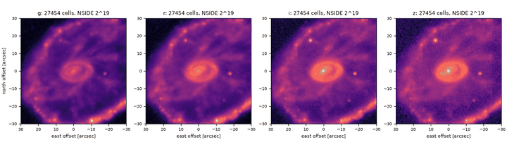
g, r, i and z sparse HEALPix maps of the Cartwheel galaxy

Each map is checked against coadd onto a planned TAN grid at the same scale:

Flux. The flux in a 25 arcsec disc agrees within 0.04 % in every band.
Pixels. The image-plane coadd, sampled at the HEALPix cell centres, differs from the map by a median of 0.02 σ.

Dense or Sparse?¶

Situation	Choice	Why
Small fraction of the sky at high resolution	`sparse=True`	only covered cells are stored
All-sky or broad survey field	`sparse=False`	a dense tensor of length \(12 N_{\rm side}^2\) indexes directly
Downstream harmonic analysis	dense	`map2alm` takes a full map

In sparse mode sky.data and sky.weight are SparseHealpixMap objects; nside_coverage sets the resolution of their coverage index (not the map resolution). nside = 4096 is already 201 million cells, so use sparse maps unless you need the full sphere.

Recipes¶

Coadd images onto a dense map¶

import torch

from torchsky.map import Observation, coadd_healpix

header = {
    "NAXIS": 2, "NAXIS1": 64, "NAXIS2": 64,
    "CTYPE1": "RA---TAN", "CTYPE2": "DEC--TAN",
    "CRPIX1": 32.5, "CRPIX2": 32.5, "CRVAL1": 150.0, "CRVAL2": 2.0,
    "CDELT1": -0.02, "CDELT2": 0.02,
}
observations = [
    Observation(data=torch.full((64, 64), value), wcs=header,
                weight=1.0, weight_is_inverse_variance=True)
    for value in (1.0, 2.0)
]
# 1.3 deg image, 0.23 deg cells (Nside 256).
result = coadd_healpix(observations, nside=256, nest=False, kernel="bilinear")

covered = result.weight > 0
assert result.data.numel() == 12 * 256**2 and int(covered.sum()) > 20
assert abs(float(result.data[covered].mean()) - 1.5) < 1e-5
print("covered cells:", int(covered.sum()), "MOC cells:", int(result.coverage_moc.uniq.numel()))

nest=False (the default) gives RING ordering; pass nest=True when the consumer expects NESTED. Kernels are nearest, bilinear, bicubic, and lanczos2 to lanczos4. The result carries data, weight, nside, nest, overlap_count (exposures per cell), and the coverage MOC.

Choose Nside¶

The cell size is about \(58.6°/N_{\rm side}\) (nside2resol). Cells up to the kernel support (two pixels for bilinear) are centre-sampled and keep the interpolation quality of the kernel. Coarser cells, down to cells larger than the whole image, are overlap-integrated: each cell is the mean of the pixels inside it, so a coarse map can be built directly from fine images.

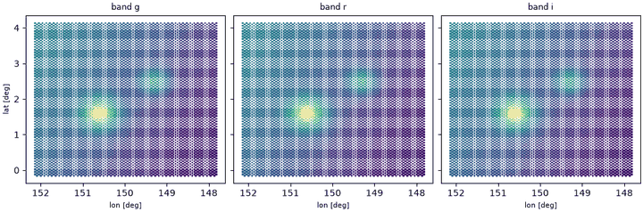
Make one map per band¶

Call coadd_healpix once per band with the same nside and ordering; cells then align across bands by construction, and a colour is a ratio of two tensors. The multiband example builds three bands from twelve overlapping tiles at \(N_{\rm side} = 1024\).

Three bands coadded onto one sparse HEALPix grid

Project a map onto an image¶

import torch

from torchsky.map import Observation, coadd_healpix, resample_healpix

header = {
    "NAXIS": 2, "NAXIS1": 64, "NAXIS2": 64,
    "CTYPE1": "RA---TAN", "CTYPE2": "DEC--TAN",
    "CRPIX1": 32.5, "CRPIX2": 32.5, "CRVAL1": 150.0, "CRVAL2": 2.0,
    "CDELT1": -0.02, "CDELT2": 0.02,
}
result = coadd_healpix([Observation(data=torch.ones(64, 64), wcs=header)], nside=256)

image = resample_healpix(result, header, method="bilinear")
covered = image.weight > 0
assert tuple(image.data.shape) == (64, 64) and int(covered.sum()) > 1000
assert torch.allclose(image.data[covered], torch.tensor(1.0))

resample_healpix takes a dense tensor (with nside=), a sparse map, or a HealpixResult, and a header, WCS, or Target. It returns a MapResult with the same data and weight contract as an image coadd. method="harmonic" interpolates through spherical harmonics; use it only when the map is band-limited and well sampled.

Bound memory on large maps¶

reduction_chunk_size (default 262,144) bounds how many sampled values are held before each reduction; lower it when many images overlap the same high-resolution cells. Dense accumulation writes each chunk into the output, and sparse accumulation grows with the covered sky, not with \(12 N_{\rm side}^2\).

Weights and uncertainty¶

Weights follow the coadd rules: relative by default, inverse variance only with weight_is_inverse_variance=True. Exposures enter in their own value semantics; for HEALPix products, surface brightness is the natural choice because every cell has the same area. Cross-cell covariance is not computed.

Pitfalls¶

Ordering. RING and NESTED maps hold the same values in different orders. Pass the ordering along with the map; most bugs show as a scrambled sky.
Frame. The map is ICRS. To compare with a Galactic HEALPix product, rotate one of them; see SHT for harmonic-space rotation.
Edge cells. With overlap integration, a cell at the edge of an exposure carries a weight equal to the covered fraction; its value is the mean of the covered part only. Check weight before treating such a cell as a full-cell average.
Zero means empty. Uncovered cells have weight == 0 and value 0; use the weight or the coverage MOC, not the value, to find them.