Fields¶

A field is a continuous model of the sky, \(F_\theta(\alpha, \delta, \lambda)\): a function you can evaluate at any right ascension, declination, and wavelength, with parameters \(\theta\). It has no pixel grid of its own. torchsky.field fits such a function to a set of images in different bands and exposures by predicting every recorded pixel through a differentiable model of the instrument and minimizing the residuals by gradient descent. The fitted field can then be rendered onto any grid: the original exposures, a new WCS image, a spectral cube, or a HEALPix map.

Two families of representations are available:

• An implicit neural representation (INR) is a small neural network that takes encoded coordinates and returns intensity. It is smooth, compact, and couples space and wavelength through shared weights.
• A spectral Power Foam divides the sky into adaptive cells (a bounded weighted Voronoi diagram), each with its own spectrum. It is local, explicit, and, with the cells fixed, linear in its spectral coefficients, so it can be solved exactly. Hybrids start an INR from a fitted Foam.

Use a field when you want one sky model constrained jointly by all bands and exposures, at native detector pixels, rather than a stack of per-band coadds; or when you need to render the same model onto several products. For a conventional stacked image, use coadds; they are also the baseline any field fit should be compared with.

How It Works¶

flowchart LR
    F["field F_θ(α, δ, λ)"] --> Q["sample at each pixel's<br/>sky footprint (WCS)"]
    Q --> B["integrate through<br/>the passband R(λ)"]
    B --> P["PSF, background,<br/>pixel response"]
    P --> M["predicted pixels μ"]
    D["image y, weight w, mask"] --> L["loss, e.g. Σ w (y − μ)²"]
    M --> L
    L -.->|"autograd"| F

For observation \(n\) and pixel \(p\), the prediction is, schematically,

with the passband \(R_n\), spatial response (PSF) \(\mathcal P_n\), pixel position \(\boldsymbol x_{np}\) from the WCS, and background \(B_{np}\). Each input is a FieldObservation: an image tensor, its FITS header as a dict, band limits or a tabulated throughput, optional weight and mask, and a PSFSpec. A Domain centres and scales sky and wavelength coordinates before they reach the model, so a float32 network never sees absolute RA and Dec. The formulation page derives the model and its assumptions.

Assumptions and Limits¶

• The sky is static during the exposures; time enters only through the observation context.
• The WCS, passbands, and noise weights are taken as calibrated. Learned PSF and background operators are available but must be constrained by calibration data (see below).
• A low training loss does not show that the reconstruction is right: compare held-out exposures, injected sources, and a classical coadd.
• On MPS, fields run in float32; fine angular structure there is not verified.

A Multi-Band Fit¶

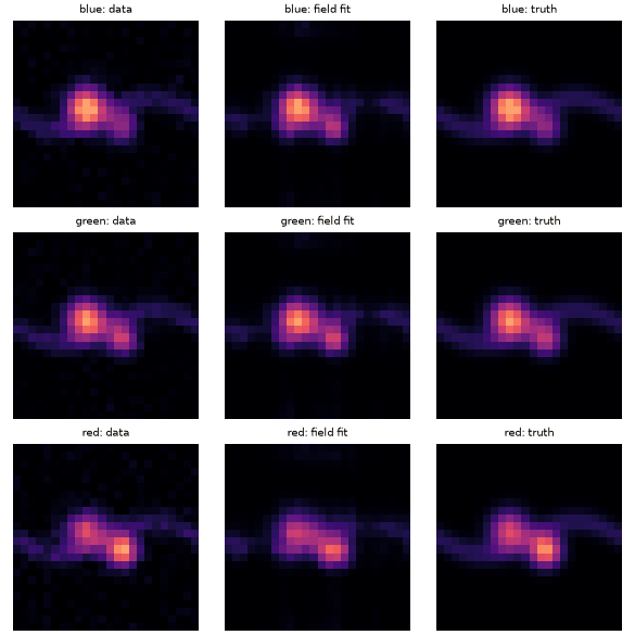
Two bands of one source, fitted by a small INR and rendered back. The multiband example does the same with three noisy bands of a two-component galaxy and masked rows:

import torch

from torchsky import field


def tangent_header(n: int = 32) -> dict:
    return {
        "NAXIS": 2, "NAXIS1": n, "NAXIS2": n,
        "CTYPE1": "RA---TAN", "CTYPE2": "DEC--TAN",
        "CRPIX1": n / 2 + 0.5, "CRPIX2": n / 2 + 0.5,
        "CRVAL1": 150.0, "CRVAL2": 2.0,
        "CDELT1": -0.05 / 3600.0, "CDELT2": 0.05 / 3600.0,
    }


gen = torch.Generator().manual_seed(0)
yy, xx = torch.meshgrid(torch.arange(32.0), torch.arange(32.0), indexing="ij")
blob = torch.exp(-((xx - 16) ** 2 + (yy - 16) ** 2) / (2 * 3.0**2))

observations = [
    field.FieldObservation(
        image=scale * blob + 0.01 * torch.randn(32, 32, generator=gen),
        header=tangent_header(),
        spectral_min=lo, spectral_max=hi, transmission_center=(lo + hi) / 2,
        weight=torch.ones(32, 32),
        band_name=name,
    )
    for scale, lo, hi, name in ((1.0, 4500.0, 5500.0, "g"), (0.8, 5500.0, 6500.0, "r"))
]

domain = field.estimate_domain(observations)
model = field.preset("fast", domain, hidden_dim=32, hidden_layers=2)
result = field.fit(observations, model, steps=30, lr=1e-2)
assert result.final_loss < result.loss_history[0]

prediction = field.render(model, observations[0])
assert prediction.shape == (32, 32) and torch.isfinite(prediction).all()

Real Data: The Cartwheel in Four Bands¶

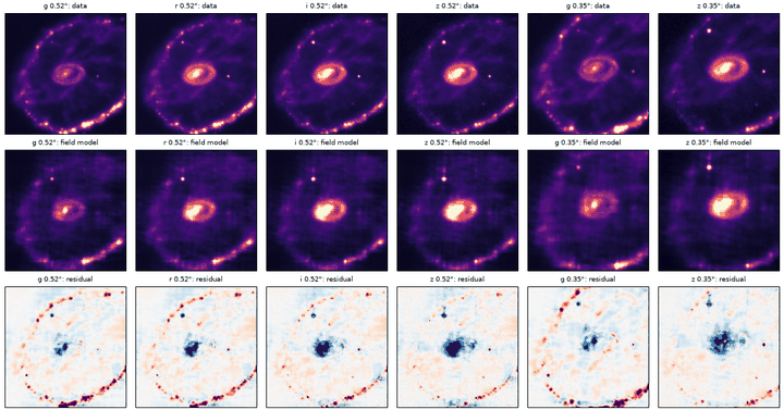
The Legacy Surveys field example fits one field to six real DECam images of the Cartwheel ring galaxy from Legacy Surveys DR10. Four bands (g, r, i, z) are sampled on a 0.524 arcsec grid, and g and z also on a 0.35 arcsec grid with a shifted centre. Each image carries its inverse-variance map, its DECam filter curve from the SVO Filter Profile Service, and a 1.1 arcsec Gaussian PSF. The two grids come from the same coadds, so the second grid tests the multi-WCS forward model, not independent data. The cutout service keeps surface brightness on every grid, which is what the field model assumes.

# fragment: the example fetches the cutouts and filter curves; see legacy_field_fit.py
import torch
import torchfits

from torchsky import field
from torchsky.filter_profiles import bandpass_from_transmission_file, field_observation_spectral_kwargs

images = torchfits.read("legacy_cartwheel_griz.fits", hdu=0).float()   # (band, y, x), nanomaggies
invvar = torchfits.read("legacy_cartwheel_griz.fits", hdu=1).float()
observations = [
    field.FieldObservation(
        image=images[k], header=header, weight=invvar[k],
        psf_spec=field.PSFSpec.gaussian(1.1 / 2.3548 / 0.524),
        **field_observation_spectral_kwargs(bandpass_from_transmission_file(f"DECam.{band}.dat", band_name=band)),
    )
    for k, band in enumerate("griz")
]                                                   # plus g and z on the 0.35 arcsec grid
model = field.preset("fast", field.estimate_domain(observations))
result = field.fit(observations, model, steps=240, lr=5e-3, num_spectral_samples=3,
                   training_patch_size=32, training_patches_per_observation=2)

After about a minute on a CPU, the model explains 74–86 % of the pixel variance in each image, and the model-to-data flux ratio is 0.94–1.09. The model reproduces the outer ring, the inner ring, the nucleus and the colour gradient between them: g − z is 1.4 mag at the nucleus and 0.4 mag on the ring. The residuals keep the star-forming knots of the ring and overshoot the nucleus: this compact network is smoother than the data. That is the gap a larger model, more steps or a learned PSF must close, and it is visible only because the example renders the model back through each observation and shows the residual. Training on 32 px patches keeps each step cheap, since a fit on full images costs the whole forward model for every pixel at every step.

Recipes¶

Build Observations From FITS Files¶

Read pixels and headers with torchfits and pass them in; tabulated filter curves from torchsky.filter_profiles give the throughput.

# fragment: needs science images, weight maps, and SVO filter files on disk
import torch
import torchfits

from torchsky import field
from torchsky.filter_profiles import bandpass_from_transmission_file, field_observation_spectral_kwargs

observations = []
for band in ("g", "r", "i"):
    image, header = torchfits.read(f"cutout_{band}.fits", hdu=0, return_header=True)
    weight = torchfits.read(f"cutout_{band}.weight.fits", hdu=0)
    spectral = field_observation_spectral_kwargs(
        bandpass_from_transmission_file(f"SDSS.{band}.dat", band_name=band)
    )
    observations.append(field.FieldObservation(
        image=image.float(), header=dict(header), weight=weight.float(),
        psf_spec=field.PSFSpec.gaussian(1.2), **spectral,
    ))

For IFU cubes, field_observations_from_ifu_cube and field_observations_from_bin_edges build one observation per spectral bin.

Choose a Model¶

field.preset gives a recommended configuration; field.model builds any kind in field.FIELD_MODEL_KINDS with explicit arguments.

A Power Foam is built from explicit cells: sites and radii in normalized tangent-plane coordinates and Legendre spectral coefficients per cell.

import torch

from torchsky import field

header = field.make_tangent_plane_header(24, 24, crval_ra_deg=150.0, crval_dec_deg=2.0, cd11=-1e-5, cd22=1e-5)
observation = field.FieldObservation(
    image=torch.zeros(24, 24), header=header,
    spectral_min=4500.0, spectral_max=5500.0, transmission_center=5000.0,
)
domain = field.estimate_domain([observation])
foam = field.model(
    "spectral_power_foam", domain,
    sites=torch.tensor([[-0.25, 0.0], [0.25, 0.0]]),         # two cells
    radii=torch.tensor([0.8, 0.8]),
    cell_coefficients=torch.tensor([[0.5, 0.1], [0.8, -0.1]]), # 2 Legendre terms each
)
assert field.render(foam, observation).shape == (24, 24)

spectral_data_budget reports how much spectral information an observation list carries and which model capacities it can support.

Render a Cube or a HEALPix Map¶

import torch

from torchsky import field
from torchsky.spectral import SpectralAxis

header = field.make_tangent_plane_header(16, 16, crval_ra_deg=150.0, crval_dec_deg=2.0, cd11=-1e-5, cd22=1e-5)
observation = field.FieldObservation(
    image=torch.zeros(16, 16), header=header,
    spectral_min=4500.0, spectral_max=6500.0, transmission_center=5500.0,
)
model = field.preset("fast", field.estimate_domain([observation]), hidden_dim=16, hidden_layers=1)

axis = SpectralAxis(torch.tensor([5000.0, 5500.0, 6000.0]), "Angstrom", "WAVE")
cube = field.render(model, target="cube", target_header=header, spectral_axis=axis, spatial_tile_hw=(8, 8))
assert cube.shape == (3, 16, 16)

target="healpix" with nside= and spectral_axis= returns (nλ, npix); spectral_chunk and spatial_tile_hw (or spatial_chunk_pixels) bound memory. Write cubes with write_cube_fits. To evaluate the field at arbitrary positions, such as catalogue sources, use field.sample(model, observation, ra_deg=ra, dec_deg=dec), which returns the field through that observation's bandpass at each (ra, dec).

Check the Fit and Save It¶

field.quality renders every observation and reports weighted residual metrics per observation and in aggregate; field.residual_product bundles prediction, data, weight, and metrics for inspection. save_artifact and load_artifact store the model with its kind, arguments, domain, and fit configuration in a directory with a JSON manifest.

Refine Exposure Poses¶

field.fit(..., refine_poses=True) adds one learnable translation, rotation, and scale per exposure. The first exposure is held fixed to remove the global shift that the poses and the sky could otherwise exchange; the fitted poses are on result.exposure_poses.

Learn the PSF and Background, in Stages¶

torchsky.map.operators provides learned PSF and background operators that plug into the same forward model through observation_operator_bundles= (for example ConditionedKernelPSF, a mixture of positive unit-sum kernels that varies with detector position, wavelength, and time). Scene, PSF, and background cannot all be free at once: a broad source can be traded for a wider PSF, diffuse emission for background. Fit in stages:

1. Fit the scene with a nominal PSF and background; keep some exposures and isolated stars out of the fit.
2. Fit a smooth background residual on source-free regions.
3. Fit the PSF on isolated stars and check encircled energy across the detector and band.
4. Refine jointly at a lower learning rate, keeping each operator anchored to its calibration, and choose capacity on the held-out exposures.

Kernel orientation and flux conventions are on the PSF conventions page.

Write Your Own Training Loop¶

field.render is differentiable, so any PyTorch loop works. torchsky.map.field.implicit_forward adds survey-level loss terms with per-survey weights and robust (Charbonnier) residuals:

import torch

from torchsky import field
from torchsky.map.field.implicit_forward import SurveyDataTerm, multi_survey_charbonnier_loss

header = field.make_tangent_plane_header(16, 16, crval_ra_deg=150.0, crval_dec_deg=2.0, cd11=-1e-5, cd22=1e-5)
observation = field.FieldObservation(
    image=torch.rand(16, 16), header=header,
    spectral_min=5000.0, spectral_max=5000.0, transmission_center=5000.0,
    weight=torch.ones(16, 16),
)
model = field.preset("fast", field.estimate_domain([observation]), hidden_dim=16, hidden_layers=1)
term = SurveyDataTerm(name="survey", observations=(observation,), loss_weight=1.0)
loss = multi_survey_charbonnier_loss(model, [term])
loss.backward()
assert torch.isfinite(loss)

Pitfalls¶

• Normalize coordinates. Custom models must subtract the field centre before casting to float32; absolute RA/Dec in float32 loses subpixel structure.
• Value semantics. Images in surface brightness and images in flux per pixel differ by the pixel solid angle; keep one convention per fit.
• Make quicklooks. Axis flips, misregistration, and tile seams show in a residual image long before they show in the loss.
• Compare with a coadd. Build coadd_multiband or a drizzled cube of the same data and read the residuals of both.

See Also¶

• Scenes: observation operators with exact adjoints.
• Likelihoods: noise models and pixel likelihoods.
• Formulation: the inverse problem behind fields.
• Examples: Cartwheel field fit on Legacy Surveys images, neural multiband field, survey split.
• Reference: torchsky.field.